Evolutionary Ecological Model of Defence Activation Disorders Via the Marginal Value Theorem

Article information

Psychiatry Investig. 2020;17(6):556-578

Publication date (electronic) : 2020 May 27

doi : https://doi.org/10.30773/pi.2020.0051

Hanson Park

Department of Anthropology, College of Social Science, Seoul National University, Seoul, Republic of Korea

Correspondence: Hanson Park, MD, PhD Department of Anthropology, College of Social Science, Seoul National University, 1 Gwanak-ro, Gwanak-gu, Seoul 08826, Republic of Korea Tel: +82-2-880-8910, E-mail: hansonpark@snu.ac.kr

Received 2020 February 8; Revised 2020 March 24; Accepted 2020 April 5.

Abstract

INTRODUCTION

Charles Darwin said that emotions such as fear are innate, highly specific to situations and the product of coordinated brain activities, and that different animal species with diverse environmental demands (or histories) have evolved unique, specialised sets of fear (or defensive) responses to maximise survival [1]. Sigmund Freud argued that humans use a defence mechanism to reduce anxiety arising from unconscious conflicts [2]. However, defence mechanisms in evolutionary psychiatry refer to adaptive responses in which individuals maximise their fitness from threatening environmental stimuli toward them. In an evolutionary context, the term fitness is a quantitative representation of natural selection or sexual selection. It refers to the ability of a genotype or phenotype to survive in the environment and produce offspring. So, as behavioural strategies to avoid risk and reduce conflicts, defence mechanisms are adaptive survival and reproductive strategies [3].

Organisms have evolved to maximise fitness by reacting appropriately to various stimuli that occur within and outside of their bodies. Emotions are the evolutionary product of the brain’s effort to regulate physiology and behaviour to gain benefits under certain conditions [4]. Humans tend to act according to individual goals, thus mapping these goals can help to estimate how emotions might have benefited potential fitness [4]. For example, in a variety of social or non-social threat situations, individuals respond in ways to protect themselves from potential or actual threats [5]. For example, individuals may use social avoidance, social withdrawal, arrested fight, blocked escape, or involuntary subordination as defensive behavioural strategies [6].

However, defensive behaviour is deeply related to negative emotions triggered by unfavourable ecological or social cues [7]. Emotions with negative valence are often considered undesirable and unhealthy. Negative emotions generally pertain to the difficulties of life, such as family death, separation, isolation, unemployment, loss of status, physical illness, social trauma, and excessive stress. Therefore, depression, anxiety or disgust are often regarded merely as unwanted consequences by undesirable internal or external happenings.

However, overactive defensive behaviours could be normal responses with adaptive value, despite their accompanying subjective uncomfortable feelings [8]. The trade-off between costs and benefits depends not on the individual’s well-being but on reproductive fitness. Even if some emotional responses are unpleasant, it could be adaptive traits if they increase the fitness of individuals or their relatives. Thus, excessive activation of some defence modules is evolutionarily inevitable [9].

Therefore, defence mechanisms can cause unpleasant responses to individuals, but cannot be considered maladaptive because they have the advantage of improving fitness [9]. According to the Error Management Theory (EMT), if the cost of false positives is less than the cost of false negatives, adaptive bias may occur to protect the individual [8].

Excessive behavioural patterns are often considered unhealthy because they cause subjective discomfort and impairment of physical, mental, and social functioning. If people show excessive negative emotion or excessive defensive behaviours, they are diagnosed as clinical psychiatric disorders. In other words, they could be not only primary evolutionary adaptive responses but also maladaptive psychological responses [10].

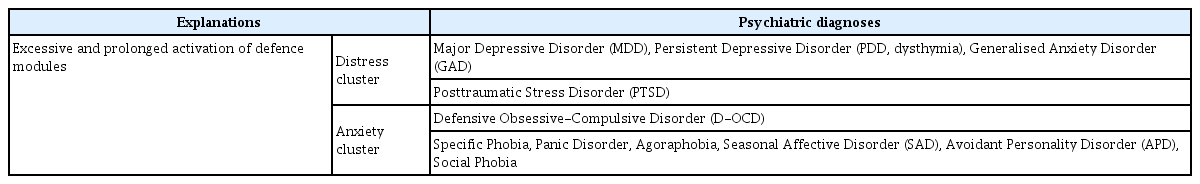
Dysfunctional behavioural patterns which are linked to negative emotions such as depressed mood, anxiety, fear or disgust may solve adaptive problems [4]. According to the Diagnostic and Statistical Manual of Mental Disorders, Fifth Edition (DSM-5), these can be broadly divided into three categories: anxiety disorders, depressive disorders, and obsessive-compulsive disorders. More specifically, these include Major Depressive Disorder (MDD), Persistent Depressive Disorder (PDD or dysthymia), Generalised Anxiety Disorder (GAD), Posttraumatic Stress Disorder (PTSD), defensive Obsessive-Compulsive Disorder (D-OCD), specific phobia, panic disorder, agoraphobia, Seasonal Affective Disorder (SAD), Avoidant Personality Disorder (APD), social phobia, and the like [11]. These are known as D-type disorders because defence behaviours are their main symptoms, although they have different clinical features, prognosis, and demographic characteristics [12].

D-type disorders, as dysfunctional behavioural patterns, can be classified into a distress cluster, which mainly shows depressive symptoms, and a fear cluster, which shows fear symptoms [13]. However, this division process is not without controversy (Table 1) [12]. For example, social avoidance, which is common in social phobia, refers to feelings of discomfort of others but also accompanies fears about face-to-face interactions. The main symptoms of MDD and GAD are depressive mood and anxiety, respectively, but most of the clinical features of these disorders are often quite indistinguishable. Also, some of the obsessive-compulsive disorders do not appear to accompany internal discomfort or fear, but it is appropriate to characterise those disorders as defence activation disorders due to the pursuit of safety and revitalization of the hate system [11,14].

Table 1.

Defence activation disorders

The prevalence of defence activation disorders is quite high. The 12-months prevalence rate of MDD, PDD (dysthymia), specific phobia, social phobia, panic disorder, GAD, and OCD was approximately 7%, 2%, 7–9%, 7%, 2–3%, 2.9%, and 1.2%, respectively. The lifetime prevalence of PTSD and APD is 8.7% and 2.4%, repectively [15].

Conversely, if defences are excessively inactive, this can be a sign of a defence inactivation disorder [16,17]. Often, defence activation disorders are referred to as D-type disorders and defence inactivation disorders as d-type disorders. The DSM-5 includes the concept of defence activation disorders but does not include the idea of defence inactivation disorders because disorders are defined in terms of impairment of subjective well-being or social functioning of individuals rather than the level of evolutionary adaptation [11]. Nonetheless, excessive inactivation of defence modules may severely impair the fitness of individuals [18]. Thus, the clinical manifestations of a manic episode of bipolar disorder could be much more harmful than those of depression even though many manic patients feel happy. Manic patients who voluntarily seek medical help are sporadic compared to depressive people who tend to seek medical help voluntarily.

The dysfunctional nature of defence activation disorders is not a matter of being unable to attend work or participate in social activities. Although it seems contrary to the argument mentioned above, that the overly activated defensive mechanisms have adaptive functions, defence activation disorders directly reduce the fitness of the individual. For example, the mortality rate for the population with MDD is 1.8 times higher than that of the general population. Moreover, the Total Fertility Rate (TFR) is only 0.9 compared to the general population [19]. In a variety of studies, infertility and affective disorders have been linked in a complex way, although the fertility rate of the general population varies from study to study [20]. There have been no reports of mental disorders with higher fertility or lower mortality rates. Is defence activation disorder only a physiological consequence of environmental stress, not an evolutionary trait?

However, defence activation disorder is not just psychological damage caused by environmental stress. In fact, the defence activation disorders run in families. The heritability of MDD is up to 37% [21]. Twins raised in different environments also show high concordance rate. The concordance rate of identical twins reaches 46–59%, while that of fraternal twins is 20–30% [22,23] when it comes to MDD. The heritability of anxiety disorders, panic disorders and social phobia ranges from 30 to 67% [24], 30 to 60%, and 13 to 76%, respectively [25].

In other words, genetic conditions that significantly lower the fitness of individuals continue at high frequencies in human populations. Although activation of defensive mechanisms contributes to the survival of individuals according to the EMT, heightened levels of defence activation seem to be related to low fitness. Despite this, defence activation still appears at a high rate in the population. It is the paradox of common, harmful, heritable mental disorders [26].

Recently, a model of balancing selection has been presented as a compelling explanation about the diversity of behavioural patterns. The model asserts that polymorphism can be maintained by natural selection with eco-evolutionary dynamics [27], even under the situation of no repetitive mutation, no gene flow, and no genetic drift. It has been supported by geneticists in the United States, including Theodosius Dobzhansky, and British ecologists [28]. The heterozygosity advantage phenomenon mentioned in the previous section is also one example of balancing selection, even though it is hard to apply to defence activation disorder.

This model can be roughly divided into the niche specialisation and the frequency-dependent selection [29,30], which are not mutually exclusive concepts.

Niche specialisation refers to the phenomenon by which each within a habitat adapts to a variety of niches [31,32]. It is the case that different genotypes are best adapted in different microhabitat environments, i.e., multiple-niche polymorphism. This phenomenon is more apparent when soft selection occurs. That is, the situation of a specific place does not affect the absolute fitness of the individual, but only the relative superiority of individuals with one particular genotype [28]. This diversifying selection by superior fitness could maintain phenotypic polymorphism and possibly explain the various activation levels of defence modules.

Habitat consists of various patches made up of different biological or non-biological conditions. An individual may occupy only a subset of the ecological niche that the entire population inhabits [33,34]. The amount of resources provided by each ecological patch depends not only on the distribution of food resources but also on the risk of attack by predators, the rapidity of resource exhaustion, the difficulty of acquiring resources, and the reproduction and survival competitiveness of populations lodging the same patches [35,36]. Therefore, each develops a variety of adaptation strategies that fit the given niches [33,34]. Since the frequency of individuals who employ in a behavioural strategy cannot be ecologically uniform in all habitats, niche specialisation can be indirect preconditions that lead to the frequency-dependent selection.

The fitness of a phenotype can be determined by the frequency of the individual exhibiting the phenotype in the population. The frequency-dependent selection is a phenomenon by which, in various ecological situations, the frequency of individuals with a particular trait is maintained continuously through interrelationships among individuals [30]. Frequency-dependent selection may be caused by interactions between individuals with different behavioural traits, or indirectly by their relative fitness to environmental conditions.

There have already been attempts to explicate MDD using the frequency-dependent selection model. Various aspects of MDD can be explained by involuntary subordinate strategies. Taken as a whole, subordinate strategies are overall associated with lower fitness but can be maintained as an evolutionarily stable strategy (ESS) depending on the frequency of population groups [37]. As more individuals become submissive, dominant individuals become more profitable. When there are more dominant individuals, the submissive individual becomes more favourable. In this condition, infrequent phenotypes have higher fitness (the inverse frequency-dependent selection). Although it is a compelling argument, it cannot apply to solitary animals. It is also questioning to explain general anxiety, fear, panic, and defensive obsession because they sometimes occur regardless of interpersonal struggle or positional competition [38]. However, the hierarchical relationship is not a prerequisite for the frequency-dependent selection. This may be caused by direct interactions between individuals with different behavioural traits but may occur indirectly, for example, by different population density among discrete ecological regions.

In the case of the ideal free distribution model, there are resource-abundant places as much as necessary, and individuals can leave and stay in any place freely. The population is increased in the affluent area. On the other hand, the population decreases in the resource-poor area. As a result, the resource acquisition rate becomes the same. Thus, the value of resources per individual in the former area and the latter area will eventually decrease equally [39]. If the population excessively grows in the resource-rich area, the individual living in a resource-poor area becomes relatively advantageous. The opposite is also exact. Depending on the amount of resources and population in the niche, the relative fitness of individuals is frequency-dependently determined.

Thus, behaviours that lead to dysfunctional responses can be adaptive behavioural strategies in the circumstance of a specific niche, and the genotype associated with the dysfunctional behavioural pattern can be maintained in a frequency-dependent manner for a long time in the gene pool. Perhaps defence activation disorders could be the result of multiple-niche polymorphism. However, this leads to the question of how emotional and cognitive features of depressive disorder, anxiety disorder, and obsessive-compulsive disorder have to do with the ecological situation.

Aaron Beck mentioned automatic, spontaneous, and uncontrollable negative thoughts about oneself, the world, and the future as one of the cognitive characteristics of depressed patients [40]. They called it the cognitive triad [41]. A similar cognitive tendency is observed in individuals with anxiety disorders [42]. Emotion, anxiety and cognition are deeply related to each other. Three cognitive distortions point to different entities, but they can be abridged in one schema. It is a belief that the ego will not get much from the world in the future. The cynical view toward the ego, the world, and the future can trigger psychomotor inhibition [41]. A negative cognitive schema leads to inhibitory behaviours such as losing earlier, staying longer and stopping seeking. So negative cognition makes the individuals avoid challenges and remain in situ.

Emotion is not only a subsequent phenomenon evoked by the cognition but also a mediator that guide the cognitive judgement. Moreover, emotions are often activated at the unconscious level, without any cognitive awareness. Evolutionally, feelings are older than the thoughts. The evolution of emotions could date back to the early stages of life [43].

In other words, emotion may also operate as superordinate cognitive programs that appraise what the ego can obtain from the world in the future, known as the average resource acquisition rate in the entire habitat [44]. It is impossible to obtain information on the resource acquisition rate of many patches in all habitats or to calculate the average value thereof. This assumption is in line with Tooby and Cosmides’s argument that emotions exist to orchestrate other subordinate cognitive programs to achieve the best consequence of any given situation [45]. For example, depression may be an emotional condition intended to rethink current behavioural strategies and curtail them if needed [46].

The benefits and costs of behavioural patterns can be quantified by using ecological currencies. However, it is usually not possible to measure, directly, the fitness consequences of a particular behaviour. The alternative is the use of proxies [47]. The resource could be a reasonable candidate for the ecological currency because the amount of resources acquired is usually linked to survival or reproduction [47]. Thus, an optimal model can be designed for how reproductive fitness diverges depending on the emotional levels, precisely defence activation level.

In this study, I tried to a mathematical model for evaluating the evolutionary fitness of individuals with defensive activation strategies that deviated from the average optimal value using the marginal value theorem. In addition, the validity and reliability of these models were verified through agent-based simulations.

METHODS

According to the MVT, the decision between the two strategies depends on the cost of moving to the new patch [48]. The patches here do not mean just spatial patches; patches are distributed in the infinite temporal and spatial space. If it provides an individual with diverse reproductive success, it should be regarded as a different patch [49]. The MVT is a model for explaining behavioural strategies that maximise the long-term acquisition rate in a patch environment where resources are widely distributed. Originally, MVT was proposed as a mathematical model to explain the optimal foraging strategy of animals, but it is also useful in explaining various human behavioural strategies [35].

Let us think of individuals in an ecological environment. Individuals who feel potential threats (such as attacks by predators, depletion of residual resources, conflicts and position competitions due to increased populations, and the shrunken prospect of reproduction) may activate defence modules [50,51]. What strategies can be employed by individuals with activated defence modules?

First, individuals can leave the niche with a high diminishing rate of return and search for a new ecological niche. For example, individuals can move to a patch with abundant resources and no threats from predators. Alternatively, they can defeat other competitors to monopolise the patch and redouble the return [34]. At any rate, achieving enough total reproductive fitness matters. In both cases, the defence mechanism need not be activated.

Second, individuals may remain at their patch for a longer time. This strategy works under the condition of gloomy prospects; in other words, ‘wait until spring.’ [34] It is the strategy of choice if the cost or risk of moving to a new patch is enormous.

In a patch occupied by an individual, if the rate of resource acquisition per unit time is reduced, it is helpful to leave and find a new patch. However, if a new promising patch is far in the distance or there is high uncertainty about the resource acquisition rate of new potential patches, staying in the current patch is a better choice [52]. The optimal moment to leave for a new patch depends on the marginal resource acquisition rate of the current patch, the average resource acquisition rate of the entire habitat, and the expected movement cost or travel time (Figure 1) [48].

Figure 1.

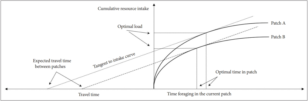
A graphical representation of the MVT (travel time reflects movement cost). MVT: marginal value theorem.

The resources of a patch (i) decrease gradually because the individuals continually pick up them. Since the individuals pick up easy-to-acquire resources first, the resource acquisition per unit time (T) - that is h_i(T_i) - also decreases gradually. Each patch has a different h_i(T_i). In Patch A with a high h_i(T_i), the rate of the resource returns declines slowly (solid line A). On the other hand, in Patch B with a low h_i(T_i), the rate of the resource returns declines rapidly (solid line B).

Then, the optimal time to leave the patch, uTi, which is the sum of the time spent in the patch (i) and travel time (t), is:

[where t=average time to search and move to the new patch; Ti=time spent in the current patch i (i=1, 2…, k)]

The mean rate of resource acquisition, that is nE_i, during the time spent in patch i and while moving to the next patch can be expressed as:

[where ET=cost per unit time to explore and move to new patches; hi (T)=the amount of resources acquired per unit time, T, from the patch (i=1, 2…, k); hi(Ti)=resource acquisition per unit time in patch i (i=1, 2,…, k)]

When the equation is differentiated by the time spent in the patch, T, the slope of the resource return obtained at a specific time in a patch is as follows:

Therefore, when the rate of resource return obtained at a specific time at a patch become equal to or smaller than the average return of the resource in the total habitat, h total (T), that is if ∂hi(T_i)/∂Ti-h _total (T) <0, the agent should leave the current patch.

When the value of ∂h_i(T_i)/∂Ti-h _total (T) approaches zero, the defence module would be activated. The reduction in the resource acquisition rate is the critical ecological pressure that directly affects the survival and reproduction of individuals. In Figure 2, it is advantageous for individuals in the patch A to stay there longer than individuals in the patch B, because the resource acquisition rate decreases more slowly in the patch A than in the patch B. In other words, the defence module should be activated more quickly and robustly in resource-poor patches (Figure 2). This logic is consistent with results of clinical studies that defence activation disorders occur more often in the unfortunate socioeconomic situations such as high competition, socioeconomic crisis, high unemployment rate, and natural disasters [53-57].

Figure 2.

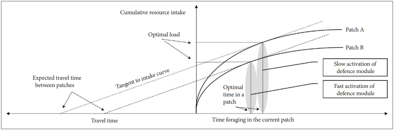
A graphical representation of the activation of defence module and the resource acquisition rate (travel time reflects movement cost).

As mentioned above, the optimal time to leave the patch is determined by ∂h_i(T_i)/∂T_i-h _total (T). The agent in the patch already knows the hi(T_i) and T_i. However, information about h _total (T), the average resource acquisition rate in a given habitat, cannot be obtained accurately at the individual level.

In Figure 3, let C_a be the initial value. Then, the x-axis value T_a, where the dashed line A touches the marginal value curve, is the optimal time to remain in the current patch or the cost of remaining in the current patch. However, the cost (or risk) of leaving to a new patch is relatively small for C_a1(T_a1<T_a). In this case, even if the cost of seeking a new patch is added, movement can increase the average return of the agent. Therefore, it is advantageous to move to another patch after T_a1, whereas the cost (or risk) of C_a2 moving to a new patch is relatively higher than that of C_a. Therefore, it is advantageous to stay longer in the current patch (T_a2>T_a).

Figure 3.

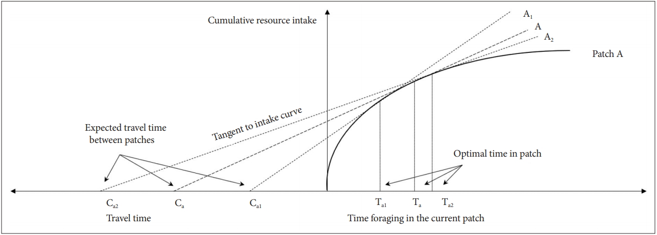
Optimal time to spent in the current patch depending on movement cost.

However, when the actual h _total (T) is the slope of the dashed line A, if the agent misinterprets it as the dotted line A₁, the agent leaves the current patch earlier than the optimal time and moves to a new patch. In this case, the agent underestimates the cost (or risk), for leaving to a new patch. By contrast, if the agent misinterprets it as the dotted line A₂, it leaves the current patch later than the optimal time. In this case, the agent overestimates the cost (or risk), for leaving to a new patch.

Let d be the weight of the individual for h _total (T). Therefore, the weight of average resource acquisition per unit time, weighted h _total (T), can be expressed as:

Here, d is assumed to be a normal distribution with an average of 1, a maximum value of 2, and a minimum value of 0. In other words, an individual in a patch will try to leave the patch when ∂h_i(T_i)/∂T_i-h _total (T)·(1-(d-1))<0. Here d>1 means that the agent is more pessimistic than the actual condition of the entire habitat, and d<1 means that the agent is more optimistic than the actual condition of the entire habitat. Thus, d is greater than 1 for D-type disorders and d is less than 1 for d-type disorders.

The primary alternate hypothesis of this study is that a range of dysfunctional behavioural strategies with different levels of defence activation can be maintained as ESS within the agent-based evolutionary simulation environments by the evolutionary mechanisms of balancing selection only when the gradient distribution of resource exists (H₁). Therefore, the null hypothesis is that a range of dysfunctional behavioural strategies with different levels of defence activation cannot be maintained in any case or can be maintained regardless of the gradient distribution of resource (H₀) within the agent-based evolutionary simulation environments.

In order to verify these hypotheses, I assume the following three environments. In the first environment, the resources are uniformly distributed both spatially (E₁). In the second environment, resources are not distributed spatially uniformly, but are randomly distributed throughout the environment (E₂). In the third environment, resources are not uniformly distributed in space, and resources are distributed in a gradient in accordance with a certain spatial tendency in the entire environment (E₃).

If a range of dysfunctional behavioural strategies with different levels of defence activation can be maintained only in E₃, the null hypothesis can be dismissed. Otherwise, I cannot prove the alternative hypothesis. Otherwise, the alternative hypothesis cannot be verified in an evolutionary simulation environment.

The agent-based model of defence activation disorders via the MVT was programmed using NetLogo [58]. Model description followed the ODD (Overview, Design concepts, Details) protocol.59,60 The abbreviations used in the model are as follows (Table 2).

Table 2.

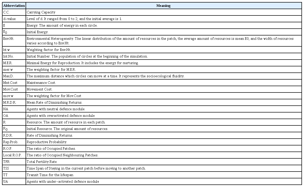
The abbreviations used in the marginal value model of defence activation disorders

ODD (Overview, Design concepts, Details) protocol

Overview

Purpose

The purpose of the agent-based model of defence activation disorders is to determine whether diverse activation levels work as ESS, even though they are sub-optimal in the context of the entire environmental condition. The model aims to demonstrate the phenomenon that the proportion of individuals with high d-value and low d-value maintains stable under various patchy environment. Additionally, the factors affecting the proportion of individuals with high or low d-value are analysed.

Entities, State Variables, and Scales

This model has two kinds of entities: the people, which are represented as circles (movable agents), and the ecological niches, which are represented squared patches (fixed agents) in the two-dimensional squared environment reflecting the entire habitat. The model is spatial: the patch consists of 1,369 square grid environments (37×37). In this model, patches with spatially unequal resource level are arrayed on a two-dimensional plane. Only one circle can be placed in a patch. Patches do not just mean the spatial place, but also refers to the various environmental conditions within entire habitat (Figure 4).

Figure 4.

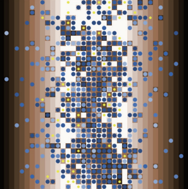
The simulated world of the model.

Each patch has two important state variables

The R₀, the R. The circle can get information about the R from the patch. The amount of resources is distributed differentially, according to Env.Ht. The distribution is vertically uniform and horizontally gradient. R₀ of patches arranged from the lowest to the highest through x-coordinates. The average amount of resource is set as 150 (at xcor 9). When Env.Ht. is 1, the resource amount of patch with xcor 0 is 300, and the resource amount of patch with xcor 18 is 0. If Env. Ht. is 0, the resource amount of patch with xcor 0 is 150, and the resource amount of patch with xcor 18 is also 150. If Env. Ht. is 2, the resource amount is distributed from -150 to 450. The details are explained again in the section of sub-models.

The circle has state variables of age, E₀, E and d-value. The Int.No. and the E₀ of the circle is set at the initial setting. A circle represents each movable agent on the interface screen, and a new-born circle is displayed in yellow for one year. Movement between patches means leaving to a new ecological patch, and the energy required to movement corresponds to Mov.Cost.

The model runs at a yearly time step. Each circle survives for up to 25 years, reflecting the reproduction period from 15 to 40 years of age. Anthropologically, children aged 15 or younger are hard to give birth without potential health problems and acquire enough resources for nurturing by themselves [61]. Resources for survival to age 15 are included in M.E.R. Also, although individuals after age 40 can increase inclusive fitness through additional production, this is purposefully disregarded for the simplification of the model. The circle of the model has no gender. Time-span of simulations reflect mainly 5 or 10 kiloyears (kyr).

Process overview and scheduling

The model includes the following actions. They are performed in the order listed at each time step. 1) Energy Acquisition and Maintenance: The circle acquires resources from the patch. The E increases by multiplying the patch’s resources by R.D.R. The default value of R.D.R. is 0.3. The R of the patch is reduced by the same amount which the circle gets. Moreover, the E of the circle falls by Mnt.Cost. If the circle’s E reaches below 0 or the age exceeds 40, the circle dies. Died circles are removed from the environment at the beginning of the next step. 2) Decision of Movement: The circle moves to another patch if the expected amount of energy acquisition on the patch is less than the expected amount of average energy acquisition in the entire habitat in addition to Mov.Cost and if E exceeds Mov.Cost [48]. At this time, the expected average amount of energy acquisition in the entire habitat is calculated by weighting the d-value of each circle on the actual amount of average energy acquisition. If the circle does not move, the TSS of it increases by 1. When a move is completed, the TSS returns to zero. 3) Movement: The circle moves randomly to one of the neighbouring patches. If there are no empty patches in 8 neighbours, the circle stays. If movement becomes successful, Mov.Cost is paid from E. 4) Decision of Reproduction: If the age is between 15 and 40 years old, the E of the circle is higher than M.E.R. weighted by (1-Rep.Prob.), and there are empty patches among neighbours, the circle breed a new offspring. The new-born circle begins the life at one-of neighbouring patches. If there are no empty neighbouring patches, the circle waits for the next chance. The d-value assigned to the newborn circle is set by multiplying the parental d-value by a randomly determined number in the distribution with an average of 1 and a standard deviation of d (SD-of-d). Here, Rep.Prob. is determined by the logistic function. Details are provided in the section of sub-models.

Details

Initialization

The model initiated with 400 circles, but the population of circles can be modified from 1 to 1,369 (Int.No.). The number 400 is an arbitrary number, but it is intended to reflect the magic number 500 of typical hunter-gatherer societies [65]. The number 400 is close to the 475 people considered as the natural reproduction population size [35]. However, because it did not reflect the population under 15 and over 40, 400 circles were supposed to be enough number above the minimum population size to withstand short-term fertility and mortality changes [66].

Circles located at the centre of each patch randomly. Colour of circles is blue; the more energetic they are, the lighter their colour is. However, new-born circles coloured yellow for one year. The initial energy level (E₀) of the circle can be adjusted up to 200, but the initial default value is a mean of 50 (0–100). The R.D.R. and M.R.D.R. of each patch can be within 0 and 1. Mov.Cost. can be set from 0 to 100, but the initial default value is 7. Mnt.Cost can be within 0 and 100, but the initial default value is 20. The Env. Ht. is 1, but it can be adjusted from 0 to 2. The C.C. can be up to 1,500, but the initial default value is 900. M.E.R. may reach 400, but the initial default value is 130. The d-value of the parent mostly determines the d-value of the offspring. The model is designed to give birth to one to three offspring for a lifespan. It reflects two to six offspring because parents in this model to give birth to a 15-year-old offspring. Indeed, childhood mortality rates in hunter-gathering communities range from 50 to 60% [67,68]. Innate d-value is determined by parent’s d-value multiplied by the number randomly selected from the normal distribution with an average of 1 and a standard deviation of d (SD-of-d). The default value of SD-of-d is 0.03.

Input data

This model uses no time series inputs.

Sub-models

(1) Energy acquisition and maintenance

Let R₀ be the initial resource amount of each patch. In each patch, the circle acquires resources as energy. Energy acquisition and Mnt.Cost are set as follows:

E1 = E0+ R0× R.D.R. (0≤R.D.R.≤1)

Each patch also loses the same amount of resources. Also, each circle loses Mov.Cost. (if move) and Mnt.Cost. When k times are repeated, the amount of final energy obtained is as follows:

Ek = Rk-1× R.D.R. - (Mov. Cost. + Mnt. Cost.), (k≥1)

Let R_k be the amount of resources remaining in the patch after k repetitions, as follows:

Rk = R0(1-∑R.D.R.nn=1) - (Mov. Cost. + Mnt. Cost.), (k≥1)

This can be reflected as follows:

En+1 = En + (Rn × R.D.R.)Rn+1 = Rn - (Rn × R.D.R.)En+1 = En  + (Rn × R.D.R.) - Mint. Cost.

(2) Gradation of resource distribution

When the coordinates of the centre patch are (0.0), the habitat has a square structure with 37 vertical and 37 horizontal patches. If the coordinates of a patch are (X, Y), it has a value of R₀: 300 minus the absolute value of X divided by 18 multiplied by 300. If the X value is 0, the resource is 300, and if the X value is 18, the resource is 0 (default). It is calculated as follows.

Rpxcor(x) = Mean. R0 × (Env. Ht. × ht.w + 1) - x×Env. Ht. × ht.w × Mean. R0 × 218

As mentioned above, the structure of the habitats is designed as a continuous torus of revolution.

(3) Movement cost

Mov.Cost is a value obtained by multiplying Mov.Cost by the average number of movements. Here, the average number of movements is determined as below. The mobility is different depending on the micro-environment, but it is simplified to be determined by the occupancy of the entire habitat. Thus, Mov.Cost is calculated as follows (sub-model 1):

∑k=0∞Mov. Cost × R.O.P.k= limn→∞∑k=0n-1Mov. Cost × R.O.P.k= limn→∞Mov. Cost.(1-R.O.Pn)1-R.O.P=Mov. Cost.1-R.O.P.

(4) Movement decision

The movement of the circle is determined as follows. If the proportion of the patches occupied by the circle is R.O.P., n= the number of all patches and Y–U([0, 1]);

age≤40, E > M.E.R.,Y>R.O.P.

and if the following conditions are satisfied, the circle moves.

R × (1-R.D.R.) - Mov. Cost.1-R.O.P.<R.D.R. × ∑1nR(pn)n×(1-(d-1))

Here, R(p_n) is the amount of resources in the n_th patch.

(5) Reproductive probability

Reproductive probability is calculated as follows. When the population (X₁) is 50% of the carrying capacity (C.C.) of the entire habitat, the likelihood of reproduction is P₁; when the population (X₂) is 100% of the C.C. of the whole habitat, the likelihood of reproduction is P₂. Then, intermediate variables A and B can be obtained as follows:

A=ln(P11-P2) - (ln(P11-P2) - ln(P21-P1)X1-X2× X1)B = D-CX1-X2

Here, Rep.Prob. for the given population number X is as follows:

Rep. Prob. = e(A + B × X)

If the object capacity is 500, P₁ is 0.7, and P₂ is 0.2, the logistic function of the probability of reproduction can be expressed as shown in the following chart (Figure 5).

Figure 5.

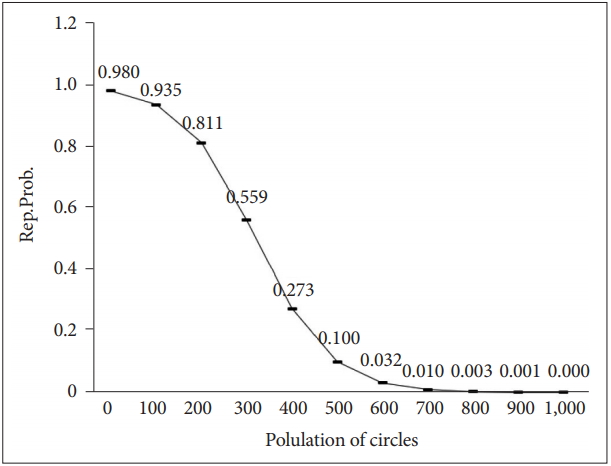
Logistic function of Rep.Prob.

(6) The circle’s d-value

In the initial state, the d-value of a circle is determined as follows:

D~U([0.5,1.5])

Each agent is classified as an overactivated agent (OA), a neutral agent (NA), or an under-activated agent (UA) depending on d-value. Therefore, they are classified as follows (SD is 0.15):

Z>1+SD : OAZ≤1+SD and Z >1 - SD : NAZ≤1 - SD : UA

Additional data about the the entire ODD (Overview, Design concepts, Details) protocol, the complete schedule of the model and whole program code are available at the Supplementary Materials (in the online-only Data Supplement).

The main parameters of this simulation model are as follows: R.D.R. (and M.R.D.R.), Env.Ht., Mov.Cost, Mnt.Cost, SD-of-d. If the setting is extreme, all circles will behave the same way. For the stable proceeding of the simulation model, the limits of each parameter were calibrated. Also, the stress tests were performed for several hundred times. Mnt.Cost is set to 20. And E₀ is set to 50. So, if net resource acquisition is 0, circles will die soon (about 3yrs after). For survival, the circle should be positioned in patches where offer at least 20 units of R every year. SD-of-d is set to 0.03. Therefore, the phenotypic variation (V_p) between parent and offspring is a maximum of 0.03. The results of the calibration are presented in the Supplementary Materials (in the online-only Data Supplement) comprehensively. The calibrated ranges of the primary parameters used in the simulation model are as follows. When parameters not listed in Table 3 are used in some simulation environment, they are described again.

Table 3.

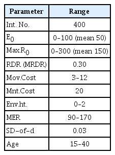
Main parameter’s value and range

RESULTS

First, the model has trustworthy reliability and feasibility. TSS was varied according to their d-value. UA, NA and OA showed different TSS. The model provided stable ranges of d-values over time. And the proportions of UA, NA and OA were also stably different across the time. The simulation model showed stable and predictable results for 5 or 10 kyr. Stress tests were conducted for 97.5 kyr, and the stability of the model is confirmed.

Second, the model yielded the expected results of niche specialisation and frequency-dependent selection at least in the simulation environment. The population density was proportional to the local resource amounts. The local d-values were distributed differentially according to the amount of resources, and the numbers of UA, NA, and OA were distributed as expected with niche specialisation. The counts of UA, NA, and OA were negatively correlated with each other in the correlation analysis.

Within the primary calibrated model environment, descriptive statistical analysis was performed, and the summaries of them are presented in the table below. The analysis of variance (ANOVA) was performed on d, population, TSS, Total Energy, and TFR to see the differences between the groups (UA, NA and OA). Bartlett’s test was performed, and each group was found to have the same variance. As will be explained later, the proportion of each subpopulation group was undoubtedly stabilised after about 0.5 to 1.5 kyr, even if an extreme initial condition is given. Therefore, data from 1,501 years to 5 kyr were collected and analysed. Most simulations were repeated for 16 times, that is 80 kyr.

Simulations were performed for 5 kyr. Several Mov.Cost and M.E.R. values were applied within the calibrated ranges. There were significant differences in d, population, TSS, total energy, age, and TFR between varied environmental conditions except for one condition. Also, there were significant differences among the three groups of UA, NA, and OA in the same environmental conditions (Table 4).

Table 4.

The d-value, populations, TSS, energy, age and TFR according to Mov.Cost and M.E.R

Especially TSS showed remarkable differences among the three subgroups (UA, NA and OA). In the environment where Mov.Cost is 7 and M.E.R. is 130, the TSS of UA was 0.2175±0.0621, but the TSS of NA was 0.4189±0.0750 and the TSS of OA was 0.8070±0.1794. In the environment where Mov.Cost is 7 and M.E.R. is 150, the TSS of UA was 0.2104±0.0559, but the TSS of NA was 0.4120±0.0586, and the TSS of OA was 0.7938±0.1638 (Table 4). This tendency suggests that the average TSS of the circle increases as Mov. Cost increases, and that the difference among the subgroups is maintained so that the sub-models of this simulation algorithm work well.

The simulation model worked reliably as the niche specialisation model. The relative proportions of UA, NA, and OA are shown in the following chart (Figure 6). The simulations were repeated for a total of 80 times. There was a slight tremor of each proportion over time, but the proportion of UA and OA was relatively low compared to NA during the most period. UA variability was higher than that of OA, but it was increased and decreased each other in an inverse way. After an average of about 400 yrs, the frequency of UA, NA, and OA entered a stable state and then continued consistently for 5 kyr.

Figure 6.

The proportion of UA, NA, and OA over time. UA: agents with under-activated defence module, NA: agents with neutral defence module, OA: agents with overactivated defence module.

If a balancing selection by a niche specialisation occurs, a stable frequency will be reached even if the initial d-value of the object is extreme. In the basic simulation setup, the d-value was set to 0.5, 1.0, and 1.5, respectively, and randomly selected one of the three d-values in each circle. So, experiments were conducted to ascertain whether d-value converged to a similar value even if it started at 0.5 or 1.5. The experiments were repeated for a total of 32 times. If the initial d-value remains unchanged or does not converge to a particular level, the assumption of balancing selection model should be rejected in the simulation environment. However, despite the extreme initial setting, the d-value converged to constant value over time. This agent-based model of defence activation disorder shows the expected outcomes of balancing selection. The relative proportion of UA, NA and OA became stable after about 1 kyr (Figure 7).

Figure 7.

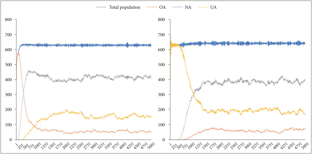
The relative proportion of UA, NA, and OA over time according to d-value. Lt.: When the initial d-value is set to 1.5 (all objects are OA), the relative proportion of UA, NA, and OA over time. Rt.: When the initial d-value is set to 0.5 (all objects are UA), the relative proportion of UA, NA, and OA over time. UA: agents with under-activated defence module, NA: agents with neutral defence module, OA: agents with overactivated defence module.

When d-value of each circle was randomly assigned from 0.5, 1.0, and 1.5 at the beginning, the standard deviation decreased gradually with time, and d-value converged to a value close to 1. The mean d-value was 0.949, and the standard deviation was 0.156. When d-value of each circle was fixedly assigned between 0.5 and 1.5 at the initial setting, the standard deviation gradually increased over time but stabilised at a similar level. And d-value also converged to a value close to 1 as well. The mean d-value was 0.939 and 0.947, and the standard deviation was 0.149 and 0.138, respectively. After about 1.5 kyr, they converged to similar patterns (Figure 8).

Figure 8.

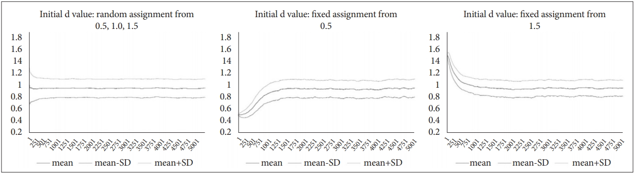
A time-series pattern of d-values and SD-of-d under three different initial settings.

As the above results, d-value of the circle stably converged in the simulation model. The initial condition affected the distribution, but after about 0.5 to 1.5 kyr, the influence of it disappeared.

Will this stable tendency persist for a very long time? The simulations were conducted under the same conditions for about 100 kyr (97.5 kyr). The results are shown in Figure 9 (Note: Until 45 kyr, four runs were averaged, and then three runs were averaged). The average of d-values for the 97.5 kyr was 0.95374+/-0.018, and the maximum and minimum values were 1.016 and 0.895, respectively. Based on the above results, it is concluded that the agent-based simulation model of defence activation disorder has fine reliability and feasibility.

Figure 9.

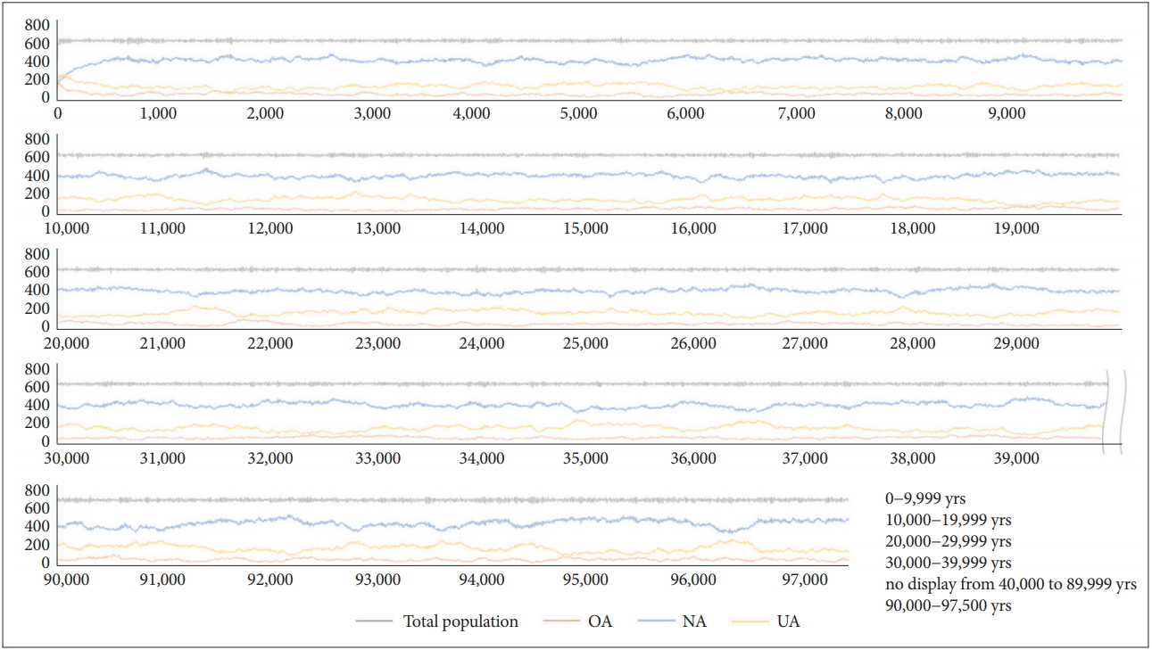
Changes in UA, NA, and OA fractions by 97.5 kyr. UA: agents with under-activated defence module, NA: agents with neutral defence module, OA: agents with overactivated defence module.

This simulation model was designed to distribute the resource amount in a direction on a two-dimensional continuous plane. In default mode, maximum R is 300, and the minimum R is 0. From 1,501 to 5 kyr, data on the location and d-value of circles according to the resource distribution were collected and analysed. The optimal d-value of the individual differs according to the resource distribution. Also, the local population densities varied depending on the amount of resources. As Mov.Cost increased, circles tended to gather in places with many resources, but the overall distribution was similar. The absolute d-value was also different, but the tendency of the difference according to the resource gradient was somewhat identical (Figure 10).

Figure 10.

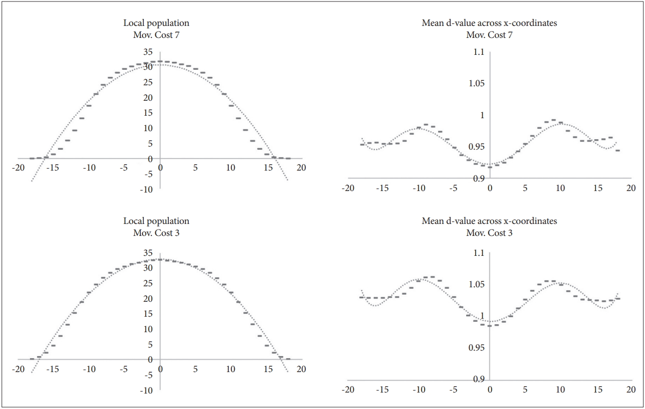
Distribution of local populations and the average d-value according to resource gradient of the x-axis (y-axis reflects the average population).

As commented in chapter 2, the circles of the simulation model have been simplified not to sense any information from patches or other circles without the R of the current patches. There is no communication and no memory. However, over the generations, the circles were specialised for local niche’s environment. The model shows the phenomenon of niche specialisation well.

On the contrary, when the resources are uniformly distributed in the whole environment, there is no local population difference (Figure 11). In addition, no regional population differences were observed when the resources were randomly distributed unequally in the overall environment (Figure 12). From these results, the null hypothesis can be rejected.

Figure 11.

Distribution of local populations and the average d-value in the environment of homogenous resource distribution.

Figure 12.

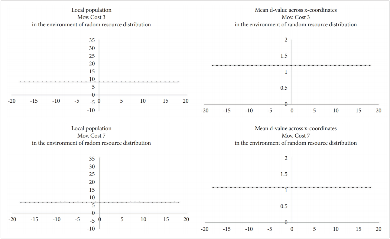
Distribution of local populations and the average d-value in the environment of random resource distribution.

As mentioned above, the population density varies according to the amount of local resources. The population density of UA, NA, and OA were different from the distribution pattern of total population density. As can be seen in Figure 13, NA was more populated in areas with high resources. However, OA was relatively populated in areas with low resources. Of course, OA has also declined at patches where resources are scarce. In contrast, UA has a relatively high population in areas with high resources. The population declined rapidly in low-resource areas, but interestingly, UA had a higher population than OA in areas with very few resources.

Figure 13.

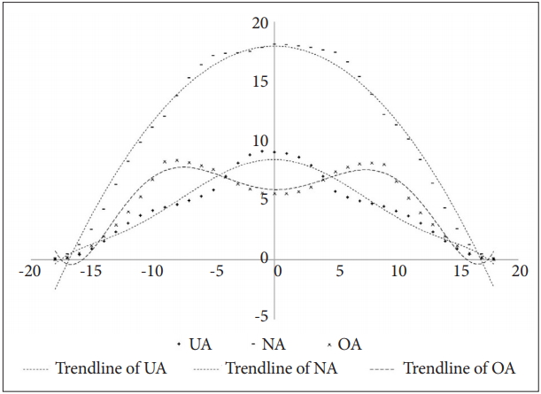
The population density of UA, NA, and OA according to resource gradient of the x-axis. UA: agents with under-activated defence module, NA: agents with neutral defence module, OA: agents with overactivated defence module.

Various optimal d-values are depending on each local environment. In other words, the diversity of defence activation level by niche specialisation was apparently observed in the simulation environment.

On the other hand, there was no difference in the local distribution of each subpopulation in the environment of homogenous or random resource distribution (Figure 14). From these results, the null hypothesis can be rejected.

Figure 14.

The population density of UA, NA, and OA in the environment of homogenous or random resource distribution. UA: agents with under-activated defence module, NA: agents with neutral defence module, OA: agents with overactivated defence module.

In an environment of Mov.Cost 7, the correlation of UA, NA, and OA population for 5 kyr was calculated (total 16 runs). NA and OA showed high negative correlations, and UA and OA also showed negative correlations. UA and NA also showed negative correlations, but the relationship was not robust when only the data after 1,500 are considered (Figure 15).

Figure 15.

The Correlation between the population of UA, NA, and OA. UA: agents with under-activated defence module, NA: agents with neutral defence module, OA: agents with overactivated defence module.

In the simulation environments where the total population is limited, UA, NA, and OA showed inverse frequency-dependent selection. OA showed relatively high negative correlations with UA and NA. OA tends to have relatively high densities in areas with low resources. However, as the population of UA or NA increased, the number of patches optimised for OA decreased, because UA and NA moved to other areas more often. Over time, an OA or UA that has moved to a patch with a low resource will be unfavourable to OA because they have relatively suboptimal behavioural strategies.

In other words, in patchy environments in which the movement is not strictly restricted, and the amount of resources is graded, the populations of individuals with various d-values would maintain inverse frequency-dependent selection.

DISCUSSION

This study is compatible with previous researches that adaptation in localised areas can evolve various behavioural patterns [30,69]. Moreover, the results also show that defence activation can be maintained as ESS at different levels in the simulation environment by balancing selection. Niche specialisation is a potent hypothesis explaining why there are various behavioural patterns. Agent-based Evolutionary Simulation model of D-type disorder is one useful way to see how niche specialisation occurs and what the environmental requirements for it are.

Beside balancing selection model, several potential evolutionary explanations have been proposed for the ultimate causations of dysfunctional behavioural patterns [70,71]. Most of them are explained in the introduction briefly. Why are so many hypotheses struggling with each other until now? There may be two reasons. First, the conceptual pluralism may reflect the complex nature of the psychological disorder [72]. Since the human mind is so complex, there have been many hypotheses about it so far. It must of necessity be so. Second, it may reflect the diverse academic interests and historical traditions about the human mind. Competing hypotheses are featured by a lack of theoretical agreement and many models are vigorously conflicting with each other [73]. A theoretical framework that can encompass many phenomena will be a solid background for building a general theory of human behaviour [74].

For an empirical evolutionary study of dysfunctional behavioural patterns, some problems must be solved [10]. First, proxy indicators as an interim measure should be established for the evolutionary study of human psychological phenomena. It is because the human mind is too complex to be quantified objectively [75]. Therefore, a human behavioural ecological approach can be useful. A simple and straightforward approach is needed. Second, appropriate currencies should be presupposed as proxy indicators. It should be universal, measurable, simulatable, and directly connected to fitness. Third, appropriate research methods are needed to observe how dysfunctional human behaviour evolved in the scale of geological time. The human mind does not remain in the fossil. Studies about contemporary hunter-gatherer studies have a variety of limitations, including small populations and external effects due to globalisation. Most of all, hunter-gatherers are not primitive survivors. Archaeological research could be useful for studying the evolution of general human psyche, but not for studying dysfunctional behavioural patterns [76].

To set the interim model, in this study, the agent-based model quantified the psychological state of anxiety, depression, and obsession as energy acquisition using the MVT. Although psychological mechanisms have not evolved solely to activate defence modules, in this study, I proposed the MVT model that can quantify defence activation level by correlating them to the appraisal weight (i.e., d-value) for the ego, the world and the future. There has been no study that have quantified the traits of dysfunctional behavioural patterns in the context of human behavioural ecology or evolutionary neuro-anthropology as far as I know.

MVT is a well-established ecological theorem and has already proven its value in explaining animal and human migration phenomena [48]. Animal studies have already been conducted using simulation models using MVT [77], and the theorem is useful for explaining the mobility of foraging society [35]. However, a simulation model of depressive disorder or anxiety disorder using MVT has not been proposed.

Of course, although MVT is a compelling ecological model, it is not possible to explain all features of the dysfunctional behavioural patterns of human with MVT. Nonetheless, simplified models can be useful in explaining aspects of complex human behaviours and evolutionary phenomena. It is not necessary to say again that the most critical element in the agent-based model is simplification [78]. In this paper, the effect of defence activation level, i.e., d-value, on ecological currency, i.e., the acquisition of energy, was studied.

In this model, the carrying capacity is used in three life activities, i.e., the movement cost, the maintenance cost, and the reproductive cost. As a result, the reproductive fitness of each can be calculated. Using ABM, it is elucidated for what evolutionary phenomena emerge in the geological timescales. As a result, this simulation model has proven to be an effective and straightforward method for evolutionary analysis of defensive activation disorders. Perhaps the results of the model can be applied to infer the phenomena of the real world.

According to the results of the study, each individual was adapted to have optimal d-value corresponding to local environmental conditions. The local optimal d-value was different from the global optimal d-value of the entire habitat. It was also observed that individuals with different d-values clustered differently depending on the local environment. In the resource-rich area, the subgroup with low defence activation level was clustered. In contrast, in resource-poor area, the subgroup with high defence activation level was clustered. The model showed that multiple defence activations level could be ESS by the mechanism of balancing selection, specifically, niche specialization, at least, in a simulated environment. A schematic diagram is shown below (Figure 16).

Figure 16.

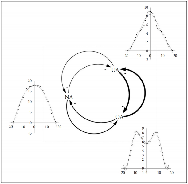
Niche Specialization and Frequency-Dependent Selection of UA, NA and OA. UA: agents with under-activated defence module, NA: agents with neutral defence module, OA: agents with overactivated defence module.

However, this phenomenon did not occur when resources were randomly distributed (not shown in this study). The random patchy environment was a prerequisite for ensuring the universality of all individuals with a global optimal d-value. If all other factors are controlled, different levels of defensive behaviour are less likely to be evolved. The Total Niche Width (TNW) of the population can be divided into the Within-Individual Component (WIC) and Between-Individual Component (BIC) [79]. All individuals in this model were premised to have the same mental and physical abilities. So Env.Ht. affect the BIC and d-value is only WIC. Specialisation occurs when WIC are much smaller than TNW or BIC is a large proportion of TNW. Therefore, under the evenly patchy environment, specialisation is hard to occur because BIC is small. However, under the resource-gradient environment, specialisation can occur quickly if free movement is limited.

In this study, the amount of resources that each individual expects depends on the resource of birthplace. Much of TNW is BIC. In the real world, however, the differences in individuals are significant. In future studies, it is necessary to investigate whether and how WIC, that is, individual traits influence the specialisation.

Also, as the population of a subgroup increased, the number of other subgroups increased. If a balancing selection occurs only by a niche specialization, the fluctuation of the proportion of individuals with different d-values will be minimised. This is because the total number of niches is limited. Since the number of niches where their d value is optimal is limited, the growth of the sub-population increases the likelihood of moving to the suboptimal area. Thus, the niche specialisation phenomenon could work as the environmental factor that maintains the proportion of subgroups with different d values in a frequency-dependent manner [30]. However, it does not appear as a predator-prey relationship, as the Lotka-Volterra equation [80] suggests. It is unclear what the negative correlation in this study has evolutionary meaning. A more sophisticated model is needed to distinguish the effects of the niche specialisation and frequency-dependent selection.

In conclusion, the simulation results offer theoretical support for the argument that defence activation levels can be maintained by multiple-niche polymorphism. The d-value by itself does not induce absolute selection pressures, but a variety of optimal d-values may appear over the long term through relative superior fitness to others in various microenvironments [28]. The multiple-niche polymorphism model could work with multiple ESS if the geographic or social gradient of the environment does not change often.

There are some limitations to this study. First, this simulation model does not have an evolutionary approach at the gene level. However, the full spectrum of genes related to behavioural traits is not yet clear, and genetic-level simulation studies are at a rudimentary level. It is also known that genetic competition is less likely to be the cause of the distinctive behavioural syndrome as the behavioural phenotype is under the control of the parliament of genes [81]. Behavioural traits are complex adaptations that are dominated by many genes. Agent-based evolutionary simulations using methodological individualism [82] could be feasible way at the present level of knowledge. Secondly, the optimal ecological model is not possible to verify why defensive behaviour is manifested in the real world [36]. However, the purpose of using the optimal simulation model is not to confirm whether individuals are behaving optimally, but to investigate qualitatively whether defensive behaviour can be explained by the criteria of optimal behaviours or constraining factors presented in the model. There may also be critical that the model and the actual defence activation phenomenon will be different. However, it is inevitable because the constraints or variables cannot, and need not, be perfect or reflect all the factors in the world [36]. The evolutionary simulation model is handy for a qualitative approach [83]. Third, there may be criticism that the optimal behaviour proposed in the model cannot be expressed in the real world. However, the ESS model with all the phenotypic gambit is a practical and useful research method that provides a robust approximation to a wide range of phenomena [84]. It is especially useful in identifying the limiting factors by ABM. The purpose of this study is to confirm the maintenance of various defence activation levels in simulation environments and to estimate the constraints. The precise optimal degree of defence activation in the microenvironment or the expected prevalence of the MDD or anxiety disorder is beyond the scope of this research. Quantitative variables have only been used as a means for qualitative approaches. The ABM itself is not designed for quantitative approach. This model should not be used to estimate the amount of defence activation, that is, how often depressive or anxiety disorders occur. As demonstrated in prior research, qualitative models are superior to quantitative models in explaining ecological phenomena in general [36].

This model shows that the fitness of the object with various d-value is relatively determined by the distribution gradient of the resources in the simulation habitat. It is due to the fixed environmental conditions [36], where each agent is located, but also by the frequency-dependent mechanism of local population density [35]. Within these conditions, there is no evolutionary significance of the so-called “the best defence activation level,” (i.e., globally ideal level mood, anxiety, fear) corresponding to the average resource value of the entire habitat. The irrational behaviour can be caused by adaptive decision process the domain of selection and the domain of testing mismatch [85,86]. The optimal level of defence activation appears relative to various conditions and circumstances, and this demonstrates there is no absolute optimal value.

This study is the first agent-based simulation study about the behavioural patterns of defence activation disorder, convert it into ecological currency by using the MVT, and reconvert it to reflect the fitness in the simulation environment to find out the ultimate causations and the relationship between d-value and ecological constraints. In particular, the model was designed using the NetLogo programming platform, which is a robust multi-agent programmable modelling environment.

A model is an intentional representation of the real world [87]. Real systems are often too complex to be implemented through experimentation. Therefore, a simplified representation of the system is required [78]. Agent-based simulations are particularly useful for behavioural and evolutionary researches. Some studies are using ABM in the field of evolutionary anthropology; however, until now, ABM has never been used for the study of evolutionary medicine. Evolutionary anthropological knowledge, experience, and research methodology may expand the scope of evolutionary psychiatry.

The MVT is a well-known theorem in human behavioural ecology and a robust explanatory framework. However, except for some preliminary attempts to study mental disorders [52], this theorem has never been used in the field of evolutionary medicine. This study will confirm the value of MVT as a functional interim model for the study of neuro-anthropology.

Defence activation disorders could be results of cognitive and emotional traits that provide a pessimistic view on the self, the world and the future. Various levels of defence could be locally adaptive behaviours optimised in a variety of ecological settings. High or low level of defence activation could act as ESS in a simulated environment. They could be dysfunctional, but the outcome of an adaptive process to discourage futile attempts and save unnecessary energy consumption.

There are some caveats in interpreting this study, but there are undoubtful advantages of evolutionary explanations of various dysfunctional behavioural patterns. Agent-based simulation studies on mental disorders are still in its infancy. I hope that the results of this research will be fruitful in the future.

Supplementary Materials

Article information Continued